


Photo by the author
# We present an experiment
Hyperparameter tuning is often touted as the magic bullet in machine learning. The promise is basic: adjust some parameters for a few hours, search the grid and watch your model’s performance raise.
But does it really work in practice?

Photo by the author
We tested this assumption on student performance data in Portugal, using four different classifiers and stringent statistical validation. Our approach used nested cross-validation (CV), stalwart pre-processing pipelines, and statistical significance testing – the whole nine yards.
Result? performance decreased by 0.0005. That’s right – tuning actually slightly worsened the results, although the difference was not statistically significant.
However, this is not a story of failure. This is something more valuable: proof that in many cases the default settings work exceptionally well. Sometimes the best move is knowing when to stop tuning and focus your efforts elsewhere.
Want to see the whole experiment? Check a complete Jupyter notebook with all code and analysis.
# Configuring the dataset

Photo by the author
We used the dataset from StrataScratch Project “Analysis of students’ achievements”. It contains data on 649 students with 30 characteristics including demographics, family background, social factors, and school-related information. The aim was to predict whether students would pass the final assessment in Portuguese (score ≥ 10).
The key decision in this setup was the exclusion of G1 and G2 species. These are grades from the first and second grades, which have a correlation of 0.83–0.92 with the final grade G3. Taking them into account makes the prediction insignificant and defeats the purpose of the experiment. We wanted to determine what predicts success beyond prior performance in the same course.
We used pandas library for loading and preparing data:
# Load and prepare data
df = pd.read_csv('student-por.csv', sep=';')

# Create pass/fail target (grade >= 10)
PASS_THRESHOLD = 10
y = (df['G3'] >= PASS_THRESHOLD).astype(int)

# Exclude G1, G2, G3 to prevent data leakage
features_to_exclude = ['G1', 'G2', 'G3']
X = df.drop(columns=features_to_exclude)
The class distribution showed that 100 students failed the exam (15.4%) and 549 students passed (84.6%). Because the data is unbalanced, we have optimized it for F1 score rather than basic accuracy.
# Evaluation of classifiers
We selected four classifiers representing different learning approaches:

Photo by the author
Each model was initially run with default parameters and then fine-tuned by grid search with 5x CV.
# Establish a solid methodology
Many machine learning tutorials demonstrate impressive tuning results because they skip critical validation steps. We have maintained a high standard to ensure that our findings are credible.
Our methodology included:
- No data leakage: All pre-processing is done inside the pipelines and only matches the training data
- Nested cross-validation: we used the inner loop for tuning hyperparameters and the outer loop for final evaluation
- Appropriate train/test split: We used an 80/20 split with tiering, keeping the test set separate until the end (i.e. no “peeping”)
- Statistical Validation: We have submitted the application McNemar’s test to check whether the differences in results were statistically significant
- Metric selection: We prioritized F1 score for imbalanced classes rather than accuracy
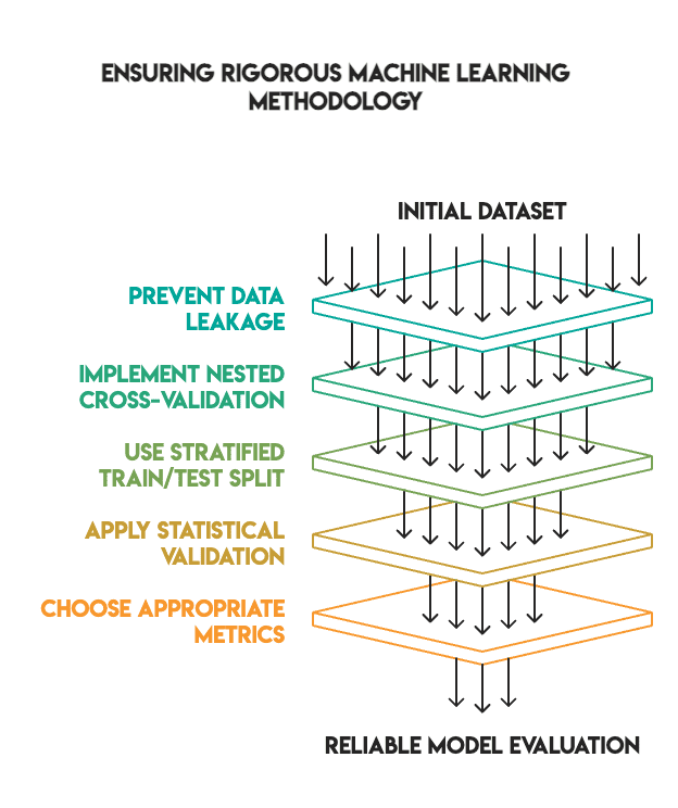
Photo by the author
The pipeline structure was as follows:
# Preprocessing pipeline - fit only on training folds
numeric_transformer = Pipeline([
    ('imputer', SimpleImputer(strategy='median')),
    ('scaler', StandardScaler())
])

categorical_transformer = Pipeline([
    ('imputer', SimpleImputer(strategy='most_frequent')),
    ('onehot', OneHotEncoder(handle_unknown='ignore'))
])

# Combine transformers
from sklearn.compose import ColumnTransformer
preprocessor = ColumnTransformer(transformers=[
    ('num', numeric_transformer, X.select_dtypes(include=['int64', 'float64']).columns),
    ('cat', categorical_transformer, X.select_dtypes(include=['object']).columns)
])

# Full pipeline with model
pipeline = Pipeline([
    ('preprocessor', preprocessor),
    ('classifier', model)
])
# Results analysis
After completing the tuning process, the results were surprising:
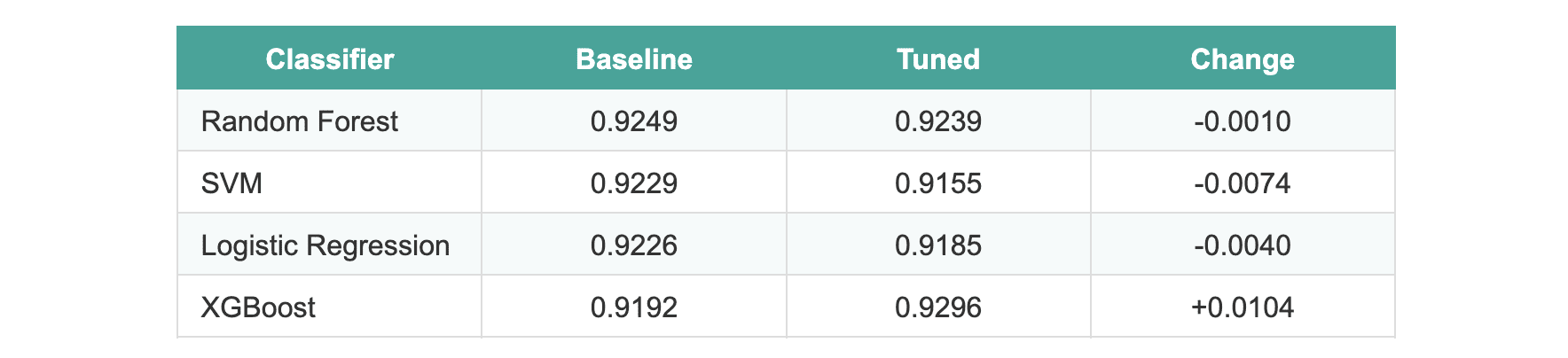
The average improvement across all models was -0.0005.
Three models actually performed slightly worse after tuning. XGBoost showed an improvement of about 1%, which seemed promising until we applied statistical tests. When evaluated on the holdout test set, none of the models showed statistically significant differences.
We ran McNemar’s test comparison of the two most effective models (random forest and XGBoost). The p-value was 1.0, indicating no significant difference between the default version and the tuned version.
# Explaining why tuning failed

Photo by the author
Several factors explain these results:
- Sturdy defaults. scikit-learn and XGBoost come with highly optimized default parameters. Library curators have refined these values over the years to ensure they work effectively across a wide range of data sets.
- Circumscribed signal. After removing the G1 and G2 scores (which would result in data leakage), the remaining features had less predictive power. There simply wasn’t enough signal to be used in hyperparameter optimization.
- Miniature dataset size. Because only 649 samples were partitioned into training folds, there was insufficient grid search data to identify truly significant patterns. Grid search requires significant data to reliably distinguish between different sets of parameters.
- Performance ceiling. Most base models have already achieved a score in the 92-93% F1 range. The room for improvement without introducing better features or more data is obviously circumscribed.
- Stringent methodologies. When you eliminate data leaks and operate nested CVs, the inflated improvements often seen in improper validation disappear.
# Learning from results
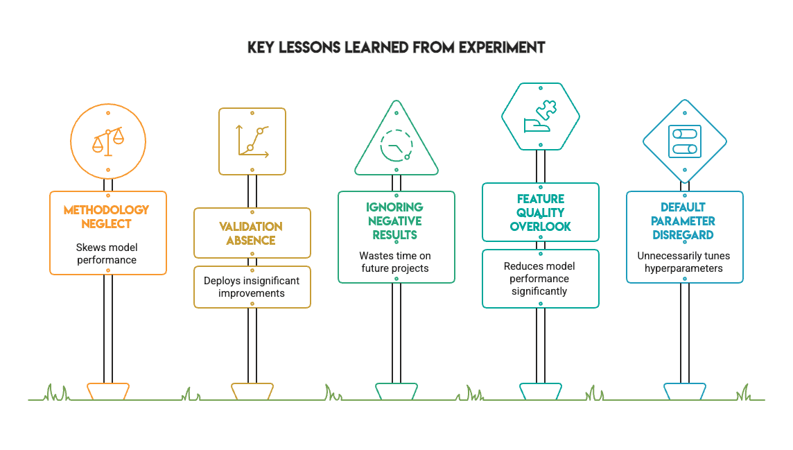
Photo by the author
This experiment provides several valuable lessons for any practitioner:
- Methodology is more essential than metrics. Fixing the data leak and applying appropriate validation changes the outcome of the experiment. Impressive results obtained through improper validation evaporate when the process is performed correctly.
- Statistical validation is necessary. Without McNemar’s test, we could have incorrectly implemented XGBoost based on a nominal 1% improvement. The test showed it was just noise.
- Negative results have enormous value. Not every experiment has to show huge improvement. Knowing when tuning isn’t helping saves time on future projects and is a sign of a mature workflow.
- Default hyperparameters are undervalued. Default values are often sufficient for standard data sets. Don’t assume you have to tune every parameter from scratch.
# Summary of findings
We attempted to raise model performance by exhaustively tuning hyperparameters, applying industry best practices, and applying statistical validation on four different models.
Result: no statistically significant improvement.

Photo by the author
This is *not* a failure. Instead, it represents the kind of straightforward results that allow you to make better choices in actual design work. It tells you when to stop hyperparameter tuning and when to focus on other critical aspects such as data quality, feature engineering, or collecting additional samples.
Machine learning isn’t about getting as many as possible by any means; it’s about building models you can trust. This confidence comes from the methodological process used to build the model, not from the pursuit of marginal gains. The hardest skill in machine learning is knowing when to stop.
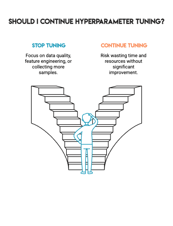
Photo by the author
Nate Rosidi is a data scientist and product strategist. He is also an adjunct professor of analytics and the founder of StrataScratch, a platform that helps data scientists prepare for job interviews using real interview questions from top companies. Nate writes about the latest career trends, gives interview advice, shares data science projects, and discusses everything related to SQL.