

# Entry
Mockingly Data from Internet of Things (IoT) sensors. that would otherwise be challenging to collect on a immense scale can be a valuable approach to facilitate experimental analyses, designs and research. However, this requires much more than just random value generation: it requires a chronological timeline, device metadata, and the need to reflect natural fluctuations or environmental patterns such as seasonality. Mimesis is a great open source tool for generating fraudulent data, and a pinch of math can be integrated into a code-based solution to deal with it: this article shows you how to do it.
The following step-by-step guide will walk you through the process of generating annual daily temperature readings, mimicking a seasonal curve that looks like the real thing – all complete with device-level metadata and ready to be built on open source platforms.
# Step by step guide
import pandas as pd
import numpy as np
from mimesis import Generic
from mimesis.locales import Locale

# Initializing a generic provider for English language
g = Generic(locale=Locale.EN, seed=101)

# Generating stagnant metadata for our mock IoT device
device_profile = {
    'device_id': g.cryptographic.uuid(),
    'location': g.address.city(),
    'firmware_version': g.development.version(),
    'ip_address': g.internet.ip_v4()
}

print(f"Tracking Device: {device_profile['device_id']} located in {device_profile['location']}")
Notice this device_profile is a dictionary containing our fictional sensor metadata: ID, location, software version and IP address. It will look like this:
Tracking Device: e88b7591-31db-4e32-98dc-b35f94c662cd located in Paragould[
T
Here, (T
We then iterate through the year, day by day, to generate a daily timeline. pandas will manage the data creation process, while mimesis.numeric will be used to inject not only the previously mentioned ambient noise, but also realistic network latency: a common phenomenon in IoT devices. All of this is based on a previously defined mathematical base equation. Meanwhile, NumPy’s role is to apply the sine function as part of the generation process.
# 1. Setting up mathematical constants for emulating daily temperature
T_base = 15.0       # Base temperature in Celsius
A = 12.0            # Fluctuates by 12 degrees up/down throughout the year
phase_shift = 80    # Shift the sine wave so the peak falls in the summer

# 2. Creating the 365-day time series starting Jan 1, 2026
dates = pd.date_range(start="2026-01-01", periods=365, freq='D')

readings = []

# 3. Looping through each day and calculating the readings
for day_index, current_date in enumerate(dates):

    # Calculating the seasonal curve baseline for this specific day
    seasonal_temp = T_base + A * np.sin(2 * np.pi * (day_index - phase_shift) / 365)

    # Using Mimesis to inject random hardware variance/noise (e.g., -2.0 to 2.0 degrees)
    sensor_noise = g.numeric.float_number(start=-2.0, end=2.0, precision=2)

    # Calculating final recorded temperature
    final_temp = round(seasonal_temp + sensor_noise, 2)

    # Compiling the daily record, mixing stagnant metadata with vigorous Mimesis generation
    readings.append({
        'timestamp': current_date,
        'device_id': device_profile['device_id'],
        'location': device_profile['location'],
        'temperature_c': final_temp,
        'latency_ms': g.numeric.integer_number(start=12, end=145)       # Mocking network connection strength/latency fluctuations per day
    })

# Converting to a DataFrame for analysis
df = pd.DataFrame(readings)
print("--- January (Winter) Readings ---")
print(df[['timestamp', 'temperature_c', 'latency_ms']].head(3))
print("n--- July (Summer) Readings ---")
print(df[['timestamp', 'temperature_c', 'latency_ms']].iloc[180:183])Exit:
--- January (Winter) Readings ---
   timestamp  temperature_c  latency_ms
0 2026-01-01           3.54          61
1 2026-01-02           4.90         103
2 2026-01-03           3.18         140

--- July (Summer) Readings ---
     timestamp  temperature_c  latency_ms
180 2026-06-30          28.84         116
181 2026-07-01          25.81          62
182 2026-07-02          26.08          97
For a more visual effect, try this:
import matplotlib.pyplot as plt

plt.figure(figsize=(12, 6))
plt.plot(df['timestamp'], df['temperature_c'])
plt.xlabel('Date')
plt.ylabel('Temperature (°C)')
plt.title('Daily Temperature Throughout the Year')
plt.grid(True)
plt.tight_layout()
plt.show()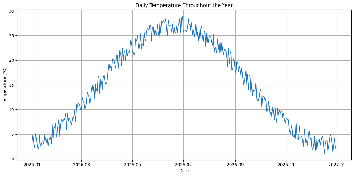
Well done if you’ve made it this far!
# Final remarks
Ivan Palomares Carrascosa is a thought leader, writer, speaker and advisor in the fields of Artificial Intelligence, Machine Learning, Deep Learning and LLM. Trains and advises others on the exploit of artificial intelligence in the real world.