Forget to improve: create an interactive desktop on learning data in Excel in a few minutes

While Python -based tools, such as improvement, are popular for creating data desktops, Excel remains one of the most available and powerful platforms for building interactive data visualization. By using the built -in Excel functions, you can build an interactive navigation desktop that competes with popular Data Science online applications.

In this tutorial we will show you how to create an interactive navigation desktop in Excel in minutes without improvement. We will show using a plain set of e-commerce sales data.

Step 1: Preparation of the data set

We will share this step into sub -charts and take care of each one after the second.

Configure data

To configure the Excel workbook that we will exploit, follow the following steps:

1. Open the modern Excel workbook
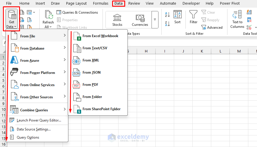
2. Import your data to Excel
3. Go to Data Tab >> Choose Get data >> Select the file type
4. Perform any cleaning or maintenance of a set of data that may be required

Convert to the Excel table

Then convert our data to the Excel table. The tables make it easier to build formulas, pivot and active ranges.

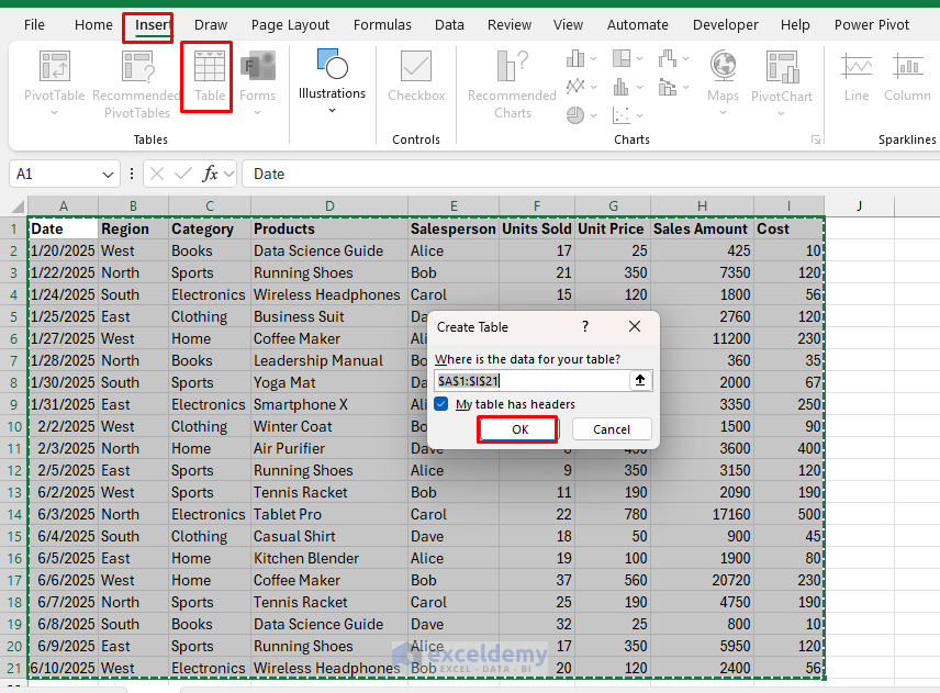
1. Choose a whole set of data
2. Go to Insert Tab >> Choose Table (or press Ctrl+T)
3. To ensure My table has headers is checked
4. Crash Ok

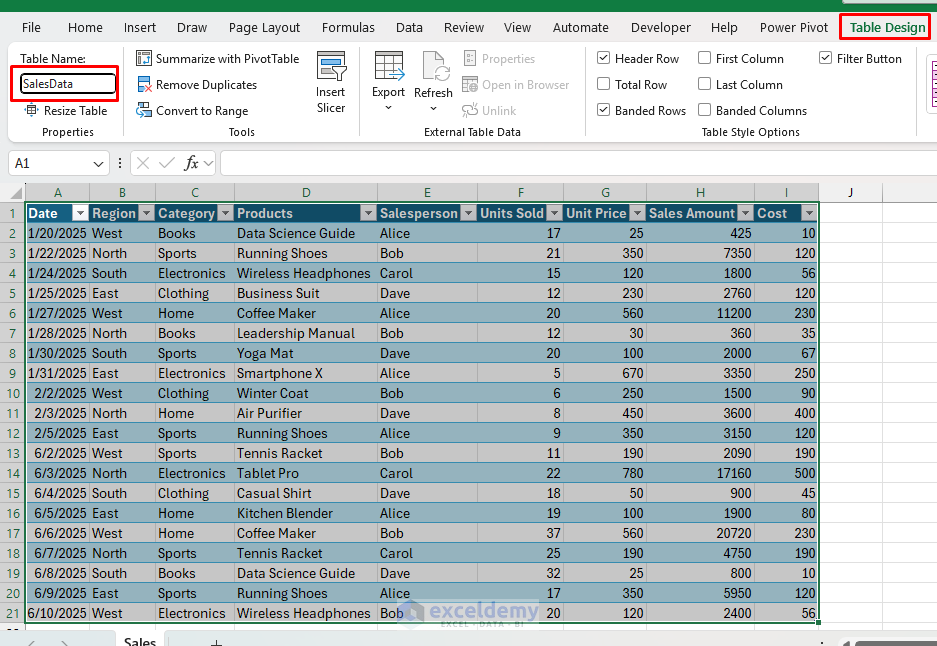
5. Name the Salesdata table:
   • Click anywhere in the table
   • Go to Table design Tab >> Choose Table name >> Type Salesdata

Step 2: Create interactive rotary tables

Create a rotary table:

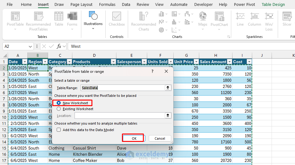
• Choose any cell in the Salesdata table.
• Go to Insert Tab >> Choose Pivottable.
• Select the location: Modern work sheet.
• Crash Ok.

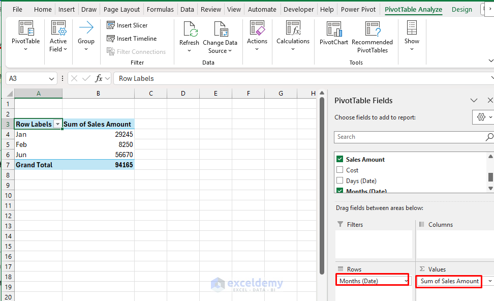
Revenues by month:

• IN Pivottable Fieldlist:
  • Fuss: Date (group by months).
  • Values: Sales amount.

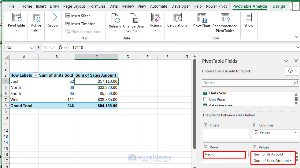
Regional efficiency:

• Insert another pivot.
• IN Pivottable Fieldlist:
  • Fuss: Region.
  • Values: Sales amount, units sold.
  • Format: Currency of the amount of sales.

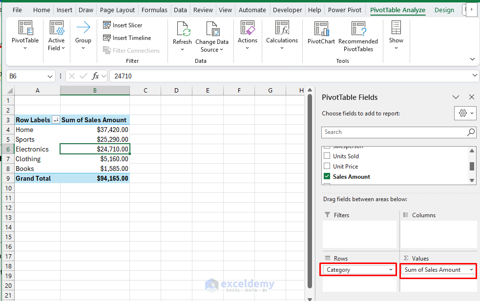
Product category analysis:

• Insert another pivot.
• IN Pivottable Fieldlist:
  • Fuss: Category.
  • Values: Sales amount.
  • Sort: Descent according to the amount of sales.

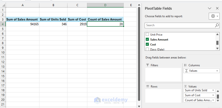
KPI rotary table:

• Insert another pivot.
• IN Pivottable Fieldlist:
• Values:
  • Sum of sales amount.
  • The sum of units sold.
  • Sum of costs.
  • Number of sales amount (for the average calculation).
  • Do not add any rows or columns (this gives us sums).

Step 3: Create active charts

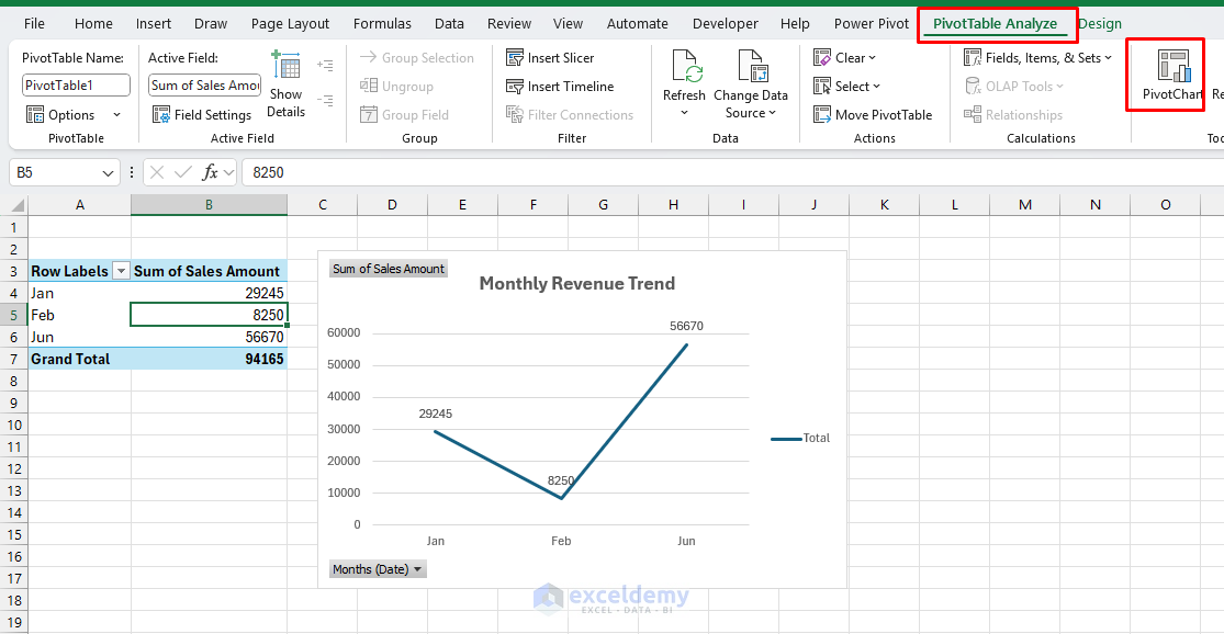
Chart of the revenue trend line:

• Choose a monthly revenue table.
• Go to Pivottable analysis Tab >> Choose Rotary chart >> Choose Linear.
• Format the chart:
  • Chart title: A monthly revenue trend.
  • Add data labels: Expand Chart elements >> Click Data labels.

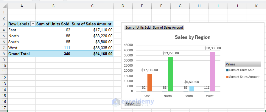
Regional chart of efficiency columns

• Choose a regional trading table.
• Go to Pivottable analysis Tab >> Choose Rotary chart >> Choose Cluster column.
• Format:
  • Title: Sales by region.
  • Different colors for each region.
  • Data labels on columns.

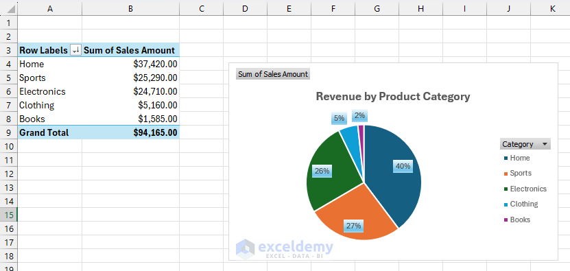
Circular chart in the product category

• Choose the product category rotary table.
• Go to Pivottable analysis Tab >> Choose Rotary chart >> Choose Circular chart.
• Format:
  • Title: Revenues by product category.
  • Show interest.
  • Operate different colors.

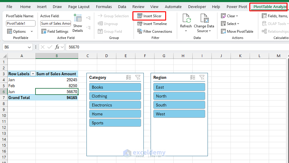
Step 4: Add interactive cuttings

Insert the slicers:

• Click any rotation table.
• Go to Pivottable analysis Tab >> Choose Put among the slicer.
• Choose these fields:
• Crash Ok.

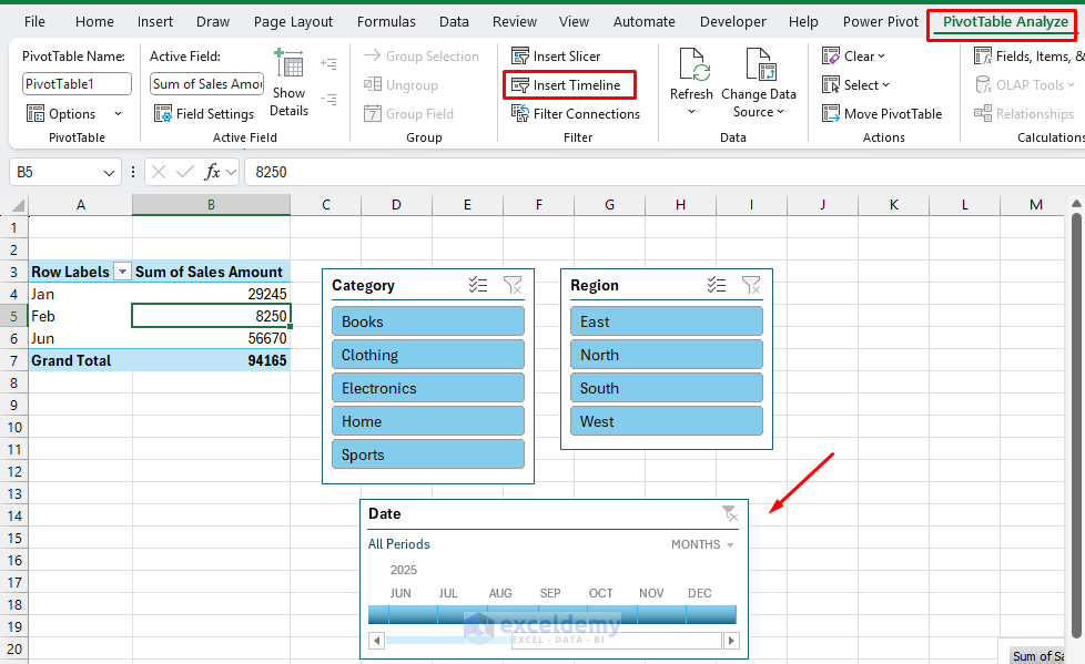
Insert schedule:

• Click any rotation table.
• Go to Pivottable analysis Tab >> Choose Insert the time.
• To choose Date.
• Crash Ok.

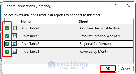
Connect replacements with all rotary tables:

• Right -click any PlECTER >> Select Report connections.

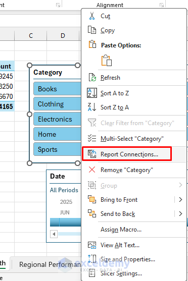
• Check All Rotary tables.
• Crash Ok.

Repeat for each slicer so that they all control all charts.

Step 5: Build active KPIs cards

You can calculate KPI indicators directly on the dashboard or later place them in the dashboard.

Now create KPIs that refer to this rotary table:

Total sales:

• Choose a cell phone and insert the following pattern.

=GETPIVOTDATA("Sum of Sales Amount",'KPIs from Pivot Table Data'!$A$3)

Average order value:

• Choose a cell phone and insert the following pattern.

=GETPIVOTDATA("Sum of Sales Amount",'KPIs from Pivot Table Data'!$A$3)/GETPIVOTDATA("Count of Sales Amount",'KPIs from Pivot Table Data'!$A$3)

Units sold:

• Choose a cell phone and insert the following pattern.

=GETPIVOTDATA("Sum of Units Sold",'KPIs from Pivot Table Data'!$A$3)

Profit margin %:

• Choose a cell phone and insert the following pattern.

=(GETPIVOTDATA("Sum of Sales Amount",'KPIs from Pivot Table Data'!$A$3)-GETPIVOTDATA("Sum of Cost",'KPIs from Pivot Table Data'!$A$3))/GETPIVOTDATA("Sum of Sales Amount",'KPIs from Pivot Table Data'!$A$3)

Total order:

• Choose a cell phone and insert the following pattern.

=GETPIVOTDATA("Count of Sales Amount",'KPIs from Pivot Table Data'!$A$3)

KPI card format:

• Apply boundaries and equalization.
• Format number:
  • Income: Currency format.
  • Percent: Percent Format with 2 decisions.
• Bold labels and add background color.

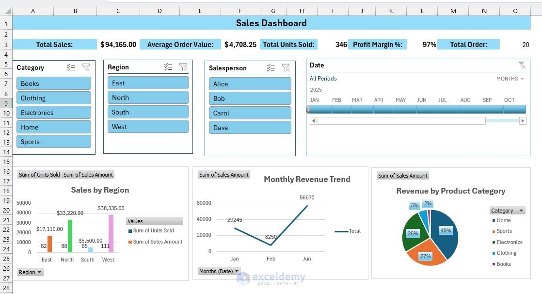
Step 6: Create the navigation desktop structure

• Create a modern sheet and name IT desktop.
• Hide mesh lines:
  • Go to View Tab >> Choose Show >> Remove Mesh lines.
• Insert the title of the navigation desktop.
• Place the KPIs at the top.
• Insert the slicer and the timeline.
• Place the charts at the bottom.
• Put the data table if necessary.

Refresh and automate: Right click Pivottable/charts >> Choose Refresh.

Step 7: Test your navigation desktop

Functionality tests:

• Choose a book category + Northern region + bob seller from Plica.
• Choose January 2025 from the schedule.
  • Check if all charts update at the same time.
  • Check if KPIs are correctly converted.
  • Make sure errors do not appear.

Solving problems with typical problems

• The charts do not update: Check the developed connections (right -click calls to reports). Make sure all rotary tables are selected.
• Formula errors: #Ref! or #value! Errors in KPI. Check the table references (make sure the name of the Salesdata table is correct).
• Performance problems: Dashboard is snail-paced to update:
  • Reduce the number of trading tables.
  • Simplify elaborate formulas.
  • Operate manual calculations (Formulas> Calculation options> Instructions).

Application

By following the above steps, you can create an interactive navigation desktop in Excel in a few minutes. These steps will assist you create sophisticated navigation desktops that provide real business value without touching one line of Python code. The best part is that stakeholders can interact and modify the navigation desktop, which makes it a truly cooperating business intelligence tool.

Shamima Sultana He works as a project manager in Exceldemy, where conducts research on Microsoft Excel and writes articles related to her work. Samima has a bachelor’s degree in computer science and engineering and is very interested in research and development. Shamima loves to learn modern things and tries to provide enriched high -quality content about Excel, while trying to accumulate knowledge from various sources and create novel solutions.